Mineral Ecology

I. THE INITIAL IDEA FOR MINERAL ECOLOGY (JUNE 2014)

The initial idea regarding chance and necessity in mineral evolution was raised during the review process of Ed Grew and Bob Hazen's paper on Be mineral evolution [Grew ES and Hazen RM (2014) Beryllium mineral evolution. American Mineralogist, 99,999-1021] by reviewer Gregor Markl, who suggested that contingency plays a role in mineral evolution. This comment evoked much further thought, including a section of the Be mineral evolution paper and the subsequent paper for the Grew volume of Canadian Mineralogist.

The Canadian Mineralogist issue was to be a secret so Hazen proposed a modest paper that considered chance and necessity in mineral evolution. But Ed found out inadvertently so Bob asked him to be a co-author, and that paper just kept expanding with new ideas into the 4-part article that introduced mineral ecology.

The original mineral ecology team:

 

 

 

 

 

 

 

 

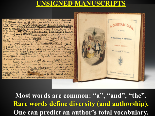
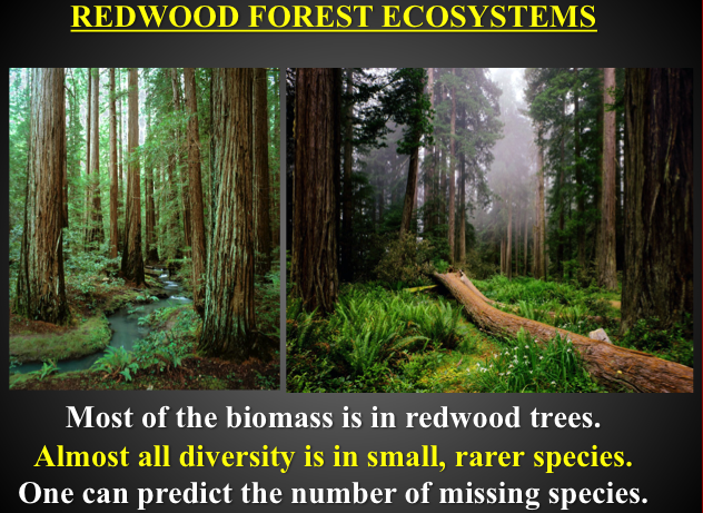
An important development was the recognition that most mineral species are rare, so minerals follow the same kind of frequency distributions as words in a book or biomass in an ecosystem. Thanks to the U. S. National Security Agency (famous for collecting and analyzing huge numbers of e-mails and phone records), the statistics of word distributions (“lexical statistics”) have been extensively studied; the authors were able to take advantage of the methods.

 

 

 

 

 

 

 

 

 

This effort got a significant boost when Hazen submitted an abstract (with severe reservations) to the October 2014 Geological Society of America meeting in Vancouver. He feared that an abstract on “mineral ecology” was so different from anything else that it would either be rejected or stuck in a “miscellany” section, to which no one would attend. Much to his surprise, the abstract was selected for the Ingerson Lecture—a “best abstract” award given by the Geochemical Society. The lecture on October 20, 2014 was the first public presentation of the ideas (though some of the key points were introduced in a keynote lecture at the International Mineralogical Society meeting in Johannesburg, South Africa on September 2^nd and a lecture at Lehigh University on September 18^th). Several subsequent mineral ecology lectures refined the ideas.

Mineral Ecology Lectures: 2014-2015

George Mason University, October 30, 2014
University of Oklahoma, November 13, 2014
American Society of Cell Biology, Annual Meeting Opening Plenary Keynote Address, Philadelphia, December 6, 2014
Indiana University, March 9, 2015
The Simons Foundation, New York, March 11, 2015
Science Museum, Munich, Germany (2nd DCO International Science Meeting), March 23, 2015 - Carbon Mineral Ecology: Predicting the "Missing" Minerals of Carbon
University of Agadir, Morocco, April 3, 2015
Geophysical Laboratory, April 13, 2015
Scripps Research Institute, April 29, 2015
Austrian Academy of Sciences, Vienna, May 18, 2015
Leibnitz Lecture, University of Potsdam, Germany, May 21, 2015
Astrobiology Science Conference, Chicago, Illinois, June 17, 2015

 

 

 

 

 

 

 

 

 

 

 

---

II. THE FIRST PAPERS (2015)

1. Hazen RM, Grew ES, Downs RT, Golden J and Hystad G (2015) Mineral ecology: Chance and necessity in the mineral diversity of terrestrial planets. Canadian Mineralogist 53(2):295-324 [pdf]

Abstract

Four factors contribute to the roles played by chance and necessity in determining mineral distribution and diversity at or near the surfaces of terrestrial planets:

1. crystal chemical characteristics;
2. mineral stability ranges;
3. the probability of occurrence for rare minerals; and
4. stellar and planetary stoichiometries in extrasolar systems.

The most abundant elements generally have the largest numbers of mineral species, as modeled by relationships for Earth’s upper continental crust (E) and the Moon (M), respectively:

Log(N_E) = 0.22Log(C_E) + 1.70  (R² = 0.34) (4861 minerals, 72 elements)

Log(N_M) = 0.19Log(C_M) + 0.23  (R² = 0.68) (63 minerals, 24 elements),

where C is an element’s abundance in ppm and N is the number of mineral species in which that element is essential. Several elements that plot significantly below the trend for Earth’s upper continental crust (e.g., Ga, Hf, and Rb) mimic other more abundant elements and thus are less likely to form their own species. Other elements (e.g., Ag, As, Cu, Pb, S, and U) plot significantly above the trend, which we attribute to their unique crystal chemical affinities, multiple coordination and oxidation states, their extreme concentration in some ore-forming fluids, and/or frequent occurrence with a variety of other rare elements—all factors that increase the diversity of mineral species incorporating these elements. The corresponding diagram for the Moon shows a tighter fit, most likely, because none of these elements, except Cu and S, is an essential constituent in lunar minerals. Given the similar slopes for Earth and the Moon, we suggest that the increase in mineral diversity with element abundance is a deterministic aspect of planetary mineral diversity. Though based on a limited number of collecting sites, the Moon’s observed mineralogical diversity could be close to the minimum for a rocky planet or moon comparable in size—a baseline against which diversity of other terrestrial planets and moons having radii in the same range as Earth and its Moon can be measured. Mineral-forming processes on the Moon are limited to igneous activity, meteor impacts, and the solar wind—processes that could affect any planet or moon. By contrast, other terrestrial planets and moons have been subjected to more varied physical, chemical, and (in the case of Earth) biological processes that can increase mineral diversity in both deterministic and stochastic ways.

Total mineral diversity for different elements is not appreciably influenced by the relative stabilities of individual phases, e.g., the broad pressure-temperature-composition stability ranges of cinnabar (HgS) and zircon (ZrSiO₄) do not significantly diminish the diversity of Hg or Zr minerals. Moreover, the significant expansion of near-surface redox conditions on Earth through the evolution of microbial oxygenic photosynthesis tripled the available composition space of Earth’s near-surface environment, and resulted in a corresponding tripling of mineral diversity subsequent to atmospheric oxidation.

Of 4933 approved mineral species, 34% are known from only one or two localities, and more than half are known from 5 or fewer localities. Statistical analysis of this frequency distribution suggests that thousands of other plausible rare mineral species await discovery or could have occurred at some point in Earth’s history, only to be subsequently lost by burial, erosion, or subduction—i.e., much of Earth’s mineral diversity associated with rare species results from stochastic processes.

Measurements of stellar stoichiometry reveal that stars can differ significantly from the Sun in relative abundances of rock-forming elements, which implies that bulk compositions of some extrasolar Earth-like planets likely differ significantly from those of Earth, particularly if the fractionation processes in evolving stellar nebulas and planetary differentiation are factored in. Comparison of Earth’s upper continental crust and the Moon shows that differences in element ratios are reflected in ratios of mineral species containing these elements.

In summary, although deterministic factors control the distribution of the most common rock-forming minerals in Earth’s upper continental crust and on the Moon, stochastic processes play a significant role in the diversity of less common minerals. Were Earth’s history to be replayed, and thousands of mineral species discovered and characterized anew, it is probable that many of those minerals would differ from species known today. 

Figure 1: A. Number of identified minerals of terrestrial origin incorporating 72 different essential chemical elements versus average upper crustal abundance of the element. The relatively low value for R² (= 0.34) can be explained by crystal chemical factors and geochemical properties of the elements.

B. Number of identified minerals of lunar origin incorporating 24 different essential chemical elements versus bulk Moon abundance of the element. Red dashed lines are ± 0.49 log units above and below the trend lines (black) based on a least square fits to all the points; i.e., 3 times more and 3 times less than the species indicated by trend lines.

 

 

 

 

 

 

 

 

 

 

Figure 2: The total number of dicotyledon plant species versus the area of islands in the Shetland Islands [after Kohn, D.D. & Walsh, D.M. (1994) Plant species richness—The effect of island size and habitat diversity. Journal of Ecology 82, 367-377]. The first-order trend of plant diversity, which increases with island area, is modified by such additional factors as the number of different habitats on each island and the proximity to other islands. Note the analogy to the figure to the right.

Figure 3: Binary phases diagrams of the (A) Hg-S (after Potter & Barnes 1978), and (B) Cu-S (after Sharma & Chang 1980), display contrasting numbers of mineral species. The Hg-S phase diagram is sparse, with only cinnabar (HgS) and its two high-temperature polymorphs hypercinnabar and meta cinnabar. By contrast, the Cu-S phase diagram is relatively crowded with at least 13 binary sulfides in the Cu-S system.

Figure 4: Observed (grey) and predicted (black) frequency spectrum for mineral distributions. The horizontal scale indicates the number of different localities, m, at which a mineral is known. The vertical scale indicates the number of different mineral species that are known from that number of localities. Thus, 1062 minerals are known from only 1 locality, whereas 569 minerals are known from only 2 localities. The observed frequencies are in close agreement with those predicted by the large number of rare event (LNRE) distribution model.

 

 

 

 

 

 

 

 

 

 

 

Figure 5: Cumulative probability of a mineral species occurring, versus the total number of localities for the mineral. For example, the probability that a mineral is found at only one locality is 22.0%, whereas the probability that it is found at 10 or fewer locations is 64.6%. Most mineral species are known from 5 or fewer localities.

Figure 6: The probability versus number of recorded localities for 4831 mineral species (data from mindat.org as of 1 February 2014): 22% of mineral species have been found at only one locality, while more than half of all mineral species are found at 5 or fewer localities. This pattern is an example of a Large Number of Rare Event (LNRE) distribution, because it is characterized by the occurrence of many mineral species with few mineral localities.

Figure 7: The LNRE model leads to predictions of the expected increase in the number of identified mineral species (upper curve). The 4831 known mineral species represent 652,856 mineral-locality pairs, as reported by mindat.org (as of 1 February 2014; vertical dashed line). As more mineral locality data are added, the number of known species is predicted to increase. This model predicts that a total of 6394 mineral species exist, assuming that current sampling and analytical procedures are employed to identify new minerals. The lower two curves are the expected numbers of mineral species reported from only 1 and from exactly 2 localities—numbers that are predicted to vary as more mineral-locality data are added. Note that as the number of mineral-locality data increase, the numbers of species known from only 1 or 2 localities are predicted to decrease.

2. EARTH'S "MISSING" MINERALS 

Hazen RM, Hystad G, Downs RT, Golden J, Pires A and Grew ES (2015) Earth’s “missing” minerals. American Mineralogist 100(10):2344–2347 PDF

Abstract

Recent studies of mineral diversity and distribution lead to the prediction of >1563 mineral species on Earth today that have yet to be described—approximately one fourth of the 6394 estimated total mineralogical diversity. The distribution of these “missing” minerals is not uniform with respect to their essential chemical elements. Of 15 geochemically diverse elements (Al, B, C, Cr, Cu, Mg, Na, Ni, P, S, Si, Ta, Te, U, and V), we predict that approximately 25% of the minerals of Al, B, C, Cr, P, Si, and Ta remain to be described—a percentage similar to that predicted for all minerals. Almost 35% of the minerals of Na are predicted to be undiscovered, a situation resulting from more than 50% of Na minerals being white, poorly crystallized, and/or water soluble, and thus easily overlooked. In contrast, we predict that fewer than 20% of the minerals of Cu, Mg, Ni, S, Te, U, and V remain to be discovered. In addition to the economic value of most of these elements, their minerals tend to be brightly colored and/or well crystallized, and thus likely to draw attention and interest. These disparities in percentages of undiscovered minerals reflect not only natural processes, but also sociological factors in the search, discovery, and description of mineral species.

Element	# Known Species	# Predicted	# Missing	% Missing	% Easily Recognized
All species	4831	6394	1563	24.4	63
Al	1005	1378	373	27.1	65
B	269	364	95	26.1	62
C	403	548	145	26.5	62
Cr	94	121	27	22.3	56
Cu	658	797	139	17.4	68.5
Mg	628	770	142	18.4	68
Na	933	1429	496	34.7	49.5
Ni	151	179	28	15.6	72
P	579	777	198	25.5	62
S	1028	1250	222	17.8	62.5
Si	1436	2002	568	28.4	61.5
Ta	60	84	24	28.6	57
Te	162	178	16	9.9	51
U	252	306	54	17.6	76
V	218	271	53	19.6	61

Table: Numbers of known mineral species; predicted number of species; inferred number of missing species; percentage of missing species; and percentage of species easily recognized in hand specimens owing to color and/or crystal form.

 

 

 

 

 

 

 

 

 

 

 

Figure 8: The number of known mineral species in Earth’s upper crust is plotted versus crustal abundance (in atom percent) for 72 essential mineral-forming elements (based on the data in Hazen et al. 2015). Most elements plot close to the linear trend defined by all elements on this log-log plot. Several rare elements that lie below the trend mimic more common elements (e.g., Ga for Al; Hf for Zr; REE for Ce or Y). Several elements that lie above the trend have multiple oxidation states and/or varied crystal chemical roles. The percentage of as yet undescribed minerals also plays a role in these deviations. This figure differs from the one above in that we switched to the more logical atom percent on the X axis.

Figure 9: (a) Frequency spectrum analysis of 4831 Earth minerals, with 652,856 individual mineral-locality data (from mindat.org as of February 2014), employed a Generalized Inverse Gauss-Poisson (GIGP) function to model the number of mineral species for minerals found at from 1 to 15 localities. (b) This model facilitates the prediction of the mineral species accumulation curve (upper curve, “All”), which plots the number of expected mineral species (y-axis) as additional mineral species/locality data (x-axis) are discovered. The vertical dashed line indicates data recorded as of 1 February 2014 in mindat.org. The model also predicts the varying numbers of mineral species known from exactly 1 locality (curve 1) or from exactly 2 localities (curve 2). Note that the number of mineral species from only 1 locality is now decreasing, whereas the number from 2 localities is now increasing, though it will eventually decrease. We predict that the number of minerals known from 2 localities will surpass those from 1 locality when the number of species-locality data exceeds ~3 x 10⁶.

 

 

 

 

 

 

 

 

 

 

 

Figure 10: (a) Frequency spectrum analysis of 151 nickel minerals with 7567 individual mineral-locality data (from mindat.org as of 1 February 2014). These data conform to a finite Zipf-Mandelbrot (fZM) function that models the number of Ni mineral species found at from 1 to 15 localities. (b) Mineral species accumulation curve for nickel minerals: Note that the number of mineral species from only 1 locality (curve 1) is now decreasing, whereas the number of minerals from 2 localities (curve 2) is close to its maximum. We predict that the number of Ni minerals known from 2 localities will surpass those from 1 locality when the number of species-locality data exceeds 15,000.

Figure 11: (a) Frequency spectrum analysis of 933 sodium minerals with 35,651 individual mineral-locality data (from mindat.org as of 1 February 2014). These data conform to a finite Zipf-Mandelbrot (fZM) function that models the number of Na mineral species found at from 1 to 15 localities. (b) Mineral species accumulation curve for sodium minerals: Note that the number of mineral species from only 1 locality (curve 1) is more than twice that of the number of minerals known from 2 localities (curve 2), in contrast to values in Figures 2 and 3.

Figure 12: The predicted percentage of missing minerals is inversely correlated with the observed percent of specimens easily recognized in hand samples owing to their color and/or crystal form. The linear regression line excludes tellurium, which may be an outlier because of the intense focus on discovering microscopic phases in thin section.

Implications: Several factors influence the differing percentages of missing minerals for different chemical elements. Physical and chemical characteristics play obvious roles. White and/or poorly crystallized phases are more likely to be overlooked. In addition, elements that form highly soluble salts, including halogens or alkali metals, or that form phases that are otherwise unstable in a near-surface environment, are less likely to be found and catalogued.

Economic factors also play a significant role, as minerals of valuable elements have received special scrutiny by mineralogists—intense study that must have biased the observed distribution. Patterns of mineral discovery also reflect the sociology of mineralogy, particularly the sensibilities of the mineral collecting community. We obtain mineral locality information from the crowd-sourced database mindat.org. It is not surprising, therefore, that brightly colored, lustrous, and/or morphologically distinct minerals are disproportionately represented owing to observational bias.

The effects of different percentages of missing minerals for different elements would have a modest but significant impact on the positions of points in Figure 1. If we considered all minerals, including Earth’s predicted missing minerals, for each element, then all points in Figure 1 would shift upward. However, points for elements with relatively well-documented minerals, including Cu, Mg, Ni, S, Te, U, and V, would shift less relative to the average, whereas the point for underdescribed Na minerals would shift more.

This study illustrates the great promise of exploiting ever growing mineral data resources, coupled with the application of powerful statistical methods. We anticipate that the discovery of new minerals, which has traditionally been based on chance finds, can transformed to a predictive science. To bring this opportunity into reality, we have commenced a series of contributions in which we will identify likely compositions and localities of Earth’s “missing” minerals.

 

3. Hystad G, Downs RT and Hazen RM (2015) Mineral Species Frequency Distribution Conform to a Large Number of Rare Events Model: Prediction of Earth’s Missing Minerals. Mathematical Geosciences 47(6):647–661 (PDF)

Grethe Hystad, from the Department of Mathematics, University of Arizona, is our mathematician and she figured out how to adapt LNRE formalisms to the mineral data. This paper from Mathematical Geosciences describes the methods in significant detail.

Abstract

We demonstrate that mineral species and their localities follow a Large Number of Rare Events (LNRE) distribution: 100 common mineral species occur at > 1000 localities, while 34% of the approved 4831 mineral species are found at only one or two localities. Models from the family of LNRE distributions fit all 4831 mineral species, as well as 112 species that incorporate the rare element beryllium. Such statistical models allow us to estimate Earth's undiscovered, mineralogical diversity. We find that both chance chemical and physical events and deterministic processes play roles in the planetary-scale evolution of mineral species. Statistical models allow us to predict the percentage of observed mineral species that would differ if Earth’s history were replayed and approximately 4831 mineral species were discovered anew with the same number of species-locality pairs. The R-code and data sets for this paper are included in an archive.

Figure 13: Observed number of localities reported for each mineral species, called the frequency, versus the rank. The mineral species are ranked according to frequencies.

 

4. Hystad G, Downs RT, Grew ES and Hazen RM (2015) Statistical analysis of mineral diversity and distribution: Earth’s mineralogy is unique. Earth & Planetary Science Letters 426(15):154–157 (PDF)

The authors were delighted when this manuscript was accepted by EPSL. It was a close thing, apparently. Mike Bickle, the editor, wrote “Probably against my better judgment I have decided to accept this paper on the grounds that I didn’t find it boring.”

Abstract

Earth’s mineralogical diversity arises from both deterministic processes and frozen accidents. We apply statistical methods and comprehensive mineralogical databases to investigate chance versus necessity in mineral diversity-distribution relationships. Hundreds of mineral species, including most common rock-forming minerals, distinguish an “Earth-like” planet from other terrestrial bodies. However, most of Earth’s ~5000 mineral species are rare, known from only a few localities. We demonstrate that, in spite of deterministic physical, chemical, and biological factors that control most of our planet’s mineral diversity, Earth’s mineralogy is unique in the cosmos.

Figure 14: The number of Be mineral species (y axis) versus the number of reported localities (m=1 to 15 localities, based on data in mindat.org as of 1 February 2014). The observed (gray) and modeled (blue) frequency spectrum of Be minerals fits a finite Zipf-Mandelbrot (fZM) Large Number of Rare Events (LNRE) distribution. Thus, half (56) of the 112 known Be mineral species (rruff.info/ima as of 1 February 2014) are known from 3 or fewer localities, whereas only 10 species are known from more than 100 localities.

Figure 15: Expected Be mineral species accumulation curves, extrapolated at 6 times the sample size (N = 6778), using Sichel's model. The upper curve indicates the expected number of distinct mineral species, E(V(N)), versus the sample size, N. The point at which the vertical dashed line intersects the x-axis denotes the current value of the sample size N = 6778, for which the current number of known Be mineral species E(V(N)) = 112. Extrapolation of the upper accumulation curve suggests that 91 Be minerals have yet to be discovered. The lower two accumulation curves represent the numbers of mineral species found at exactly 1 and 2 localities, respectively.

Figure 16: Rank versus probability that a Be mineral species in the population of 203 Be species will be present at least one time in a sample with N = 6778, where N is the number of Be mineral species-locality data.